Goal
The model server in the last post loaded a 14 MB file from its own container image. Real model servers and training jobs read much more, from places that are not on the machine they run on. I wanted to measure how fast data arrives from three of those places on this cluster: a local disk, a shared NFS directory, and an S3-style object store. I also wanted to see what the numbers look like when I repeat the same test.
This is the second post in Part 4. There are no GPUs and no real network fabric in this lab, so the results describe three small VMs on one host.
Terms used in this post
These build on the earlier glossaries.
- Sequential read or write: a file read or written in order, in large blocks. Typical for loading a model or a dataset.
- Random read or write: small reads or writes at scattered positions. Typical for a database or many small files.
- Throughput: megabytes per second moved.
- IOPS: input/output operations per second, the number of reads or writes completed.
- Queue depth: how many operations are in flight at once. At depth 1 each operation waits for the last.
- Direct I/O: reads and writes that skip the operating system’s file cache, so the test measures the storage path and not the cache on this machine.
- Page cache: memory the operating system uses to keep recently used file data.
- NFS: a protocol that lets one machine export a directory and others mount it as if it were local.
- Object storage and S3: storage where data is whole objects fetched by name over HTTP, using the S3 API that Amazon defined and others copy.
- MinIO: an open source server that speaks the S3 API.
- fio: a tool that generates read and write loads and reports throughput, IOPS and latency.
What I built
Three paths to the same kind of data, each tested from a reader on lab-node1.
- Local disk. A file on the VM’s own virtual disk.
- NFS. The
/shareddirectory from Part 1.slurm-ctlexports it,lab-node1mounts it with NFS version 4.2 and 512 KiB read and write sizes. The export is synchronous. - Object storage. A single MinIO pod on
lab-node2, storing data in an emptyDir on the node’s disk. A Python reader using the boto3 library runs as a Job, once onlab-node1and once onlab-node2, so I could compare a read from another VM with a read on the same VM.
 Diagram: where the reader, the NFS server and the MinIO pod run.
For the local and NFS paths I used fio with a 1 GiB file, direct I/O, and 15 seconds per test. For MinIO I wrote a short Python reader. The VMs are amd64 and I have no registry, so I built the MinIO image on another machine from its source repository, with the Go toolchain, and imported it onto the node as a file. It carries no release version, so I cannot say which MinIO release it is. I could not pull the official image from the public registries.
How it works
fio opens a file on the path under test and issues reads or writes at a chosen block size and queue depth, then reports throughput, IOPS and the latency percentiles. The S3 reader does the same kind of work over HTTP: it uploads a 1 GiB object, reads it back in one stream, reads 4 KiB ranges at random one at a time, and writes and reads 500 objects of 100 KiB.
Everything crosses a virtual network on one physical host. NFS traffic between two VMs, or between a pod and MinIO on another VM, never leaves that host.
Commands and results
Local disk against NFS. I ran each test twice from lab-node1. The two runs agreed within a few percent except where noted.
| Test | Local disk | NFS |
|---|---|---|
| Sequential write, 1 MiB blocks (MB/s) | 3130, 2614 | 589, 617 |
| Sequential read, 1 MiB blocks (MB/s) | 3482, 3491 | 2344, 2344 |
| Random read, 4 KiB, queue depth 1 (IOPS) | 9482, 9414 | 6804, 6843 |
| Random read, 4 KiB, queue depth 16 (IOPS) | 101,522, 100,075 | 23,986, 23,729 |
| Random write, 4 KiB, queue depth 1 (IOPS) | 15,899, 15,748 | 650, 645 |
At queue depth 1, the median latency of a random read was 0.09 ms on the local disk and 0.13 ms over NFS. A random write was 0.05 ms locally and 1.22 ms over NFS. The write difference is the largest in the table: with a synchronous export the server has to commit each write before it answers. I did not try an asynchronous export, so I cannot say how much of the gap that setting explains.
The local figures are much higher than any physical disk gives, so the hypervisor is probably caching or the backing store is very fast. I treat them as numbers for a virtual disk, not for hardware. The NFS sequential read of 2344 MB/s came from a file that had just been written, so it probably came from the server’s memory. Another sequential read test later gave from 554 to 1872 MB/s from one client, with the same setup.
Several readers at once. Model servers often start together, so I read the same 1 GiB file over NFS from both compute nodes at the same time. Each pair below is one run, in MB/s.
| Run | One node alone | Both nodes at once (each) | Total |
|---|---|---|---|
| 1 | 554 | 1075 and 1124 | 2199 |
| 2 | 1872 | 690 and 687 | 1377 |
| 3 | 1013 | 543 and 527 | 1070 |
The total did not stay the same from run to run, and it did not double: it fell from 2199 to 1070 MB/s over three runs. Both readers pulled from one server over a shared host, and the server’s file cache, described below, changes between runs, so I would not read one total as a stable figure.
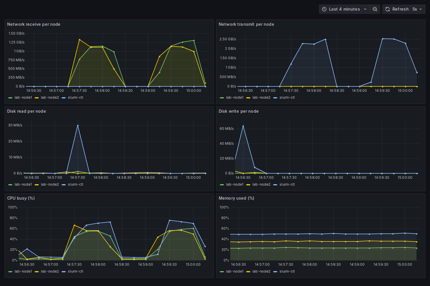 Screenshot: a second round of the parallel read with a Grafana dashboard open. The controller, which exports the share, sends up to about 2.5 GB/s while each compute node receives about 1.1 to 1.3 GB/s. CPU on all three nodes rises with the transfers.
In that second round, three runs gave 1327 and 1303, 1334 and 1299, and 1340 and 1297 MB/s for the two nodes, a total of about 2600 MB/s. That is higher than any total in the table. The file had just been written on the server, and Linux keeps the data of files it reads or writes in the page cache (kernel documentation), so the server probably sent it from memory and not from disk, which raises the ceiling (my inference).
MinIO. Three runs from each reader, with MinIO on lab-node2. Ranges are lowest to highest.
| Test | Reader on lab-node1 | Reader on lab-node2 (same VM) |
|---|---|---|
| Put one 1 GiB object (MB/s) | 81 to 153 | 92 to 200 |
| Get it back in one stream (MB/s) | 103 to 205 | 196 to 873 |
| Random 4 KiB ranged get, one at a time (IOPS) | 71 to 252 | 73 to 116 |
| Put 500 objects of 100 KiB (per second) | 10 to 54 | 20 to 24 |
| Get 500 objects of 100 KiB (per second) | 79 to 546 | 101 to 625 |
In most tests the first run was the fastest. The median time for one 4 KiB ranged get was 3.2 ms in the first run from lab-node1 and about 12 to 13 ms in four of the other five runs, including two from the same VM. The first same-VM run gave 7.7 ms. The reader on the same VM as MinIO was not reliably faster.
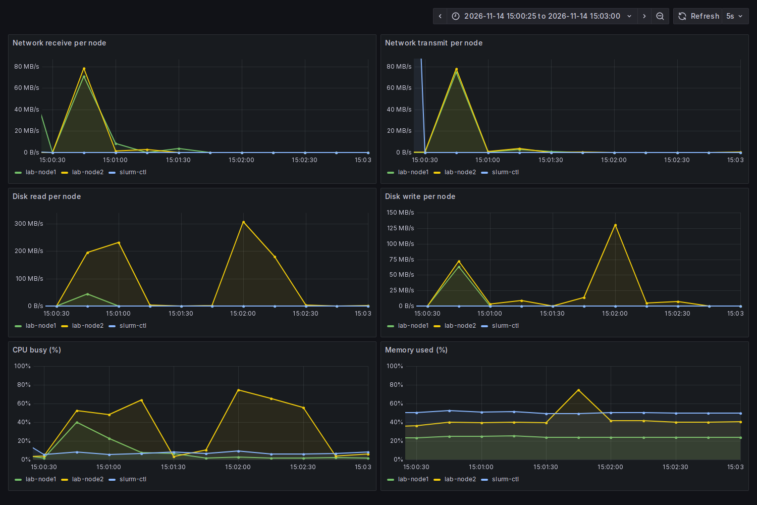 Screenshot: a second round of the MinIO runs, first from
lab-node1 and then from lab-node2, where MinIO runs. The first run shows network traffic into lab-node1. The second shows none, because the reader and MinIO share a VM, and shows lab-node2 reading the disk at up to about 300 MB/s with CPU near 75%.
Several of the second-round numbers fell outside the ranges in the table. The 1 GiB put ran at 218 MB/s from lab-node1 and 187 MB/s from lab-node2, and the 4 KiB ranged get at 323 and 334 IOPS.
Challenges
- The same test gave answers several times apart. The MinIO small-object put rate went from 54 to 10 per second from one reader, and the NFS sequential read from 554 to 1872 MB/s. The nodes share one host, so another VM’s activity could be part of it, and I did not isolate the cause. In a fleet, a single benchmark run is not an acceptance result. I would repeat it, keep the range, and set a threshold from that range.
- Shared storage did not give each reader its share. When two nodes read the same file at once, the total moved between 1070 and 2199 MB/s. A model that every new pod loads from one NFS server turns the server into the part that decides how fast a rollout goes, and I measured it only with two readers.
- A dependency I could not pull. The object store I planned to use was not available as an image I could pull, so I built it from source. That works for a lab but the result has no release number, and a fleet needs to know exactly which build runs. The lesson for operations is to mirror the images a platform depends on, with fixed versions, in a registry you control.
What this lab cannot show is real network limits, many clients, large datasets that do not fit in memory, or storage hardware.
Differences with a production setup
- Disks and network. These are virtual disks and a virtual network on one host, probably with caching underneath. Real storage has a physical device, a switch and often a 100 Gb link.
- Object store. One MinIO pod on a node’s disk, with no redundancy. Production object storage spreads data over many machines with erasure coding or replication.
- Shared file systems. NFS from a single server is common for small clusters. Large training clusters often use a parallel file system such as Lustre or object storage with a local cache, so that many nodes read in parallel.
- Client. A single-threaded Python reader sets its own limit. A latency of 12 ms for a 4 KiB read says more about that client and HTTP than about the storage, and I did not test with several parallel readers on MinIO.
- Data size. A 1 GiB file fits in memory on the server. Datasets of hundreds of gigabytes behave differently.
FAQ
What is the difference between a file system and object storage?
A file system is a tree of directories you can read at any offset and update in place. Object storage keeps whole objects under a name, fetched over HTTP. It scales out more easily, and it is slower for small random reads.
Why use direct I/O in the tests?
Without it, the second read of a file comes from memory and says nothing about the storage. Direct I/O skips that cache on the machine doing the test, though the NFS server’s cache can still affect the result.
Why is a write over NFS so much slower than a read?
In this setup the server commits each write before it replies, so every write waits on the server. Reads can be served from its memory. I did not compare with an asynchronous export.
Why report ranges and not an average?
The runs differed too much for one number to describe them. The lowest and highest values show what a reader might see.
Next
Take the quiz to test your understanding: Part 4 quiz
Part 4 continues: running Ray on the cluster and measuring a small data pipeline with one, two and three workers.
Comments