Goal
An ordinary server hall draws a load that changes slowly, as users come and go. A hall of GPUs training one model does not. Every GPU does the same work at the same time, then they all wait for each other and exchange results, and then they all start again. The power the hall draws follows that rhythm, and the source behind the hall sees it.
This post models that. I write down a load profile for 240 servers with eight GPUs each, run it through a source that smooths what it follows, and measure what the storage in between has to do. The model is a toy. It has the right shape and the right questions, and the numbers are mine.
Terms used in this post
- Synchronized load: many loads that change power at the same moment because they are working on the same job.
- Iteration: one training step, a compute phase at high power followed by a short phase of exchanging results at lower power.
- Checkpoint: a pause in which the job saves its state and the GPUs idle for a while.
- Ramp rate: how fast the power a site draws changes, in kilowatts or megawatts per second. Some utilities set limits on it.
- Smoothing: making the power the source supplies change more slowly than the load does.
- Energy storage: a battery, supercapacitor or capacitor bank that supplies the difference between the load and the smoothed source.
- Time constant: for a first-order filter, how long the output takes to cover about 63 percent of a step.
- Oscillation: a repeating swing in power, described by its frequency and size.
- Dynamic power range: the size of the short-term swing a site is allowed to produce.
What I built
bmc/gpu_load.py, a script for a hall of 240 servers with eight GPUs each, 1,920 GPUs in all.- An assumed load profile. Each GPU draws 700 W when busy and 100 W when waiting. The rest of each server draws a constant 4 kW. An iteration lasts 1.5 s with 1.1 s of compute. A checkpoint at 30 s idles every GPU for 10 s.
- A source model that follows the load through a first-order filter, so its power changes slowly. Storage supplies whatever the source does not.
- Four settings of the filter time constant: none, 1 s, 5 s and 20 s. For each I measure the swing the source still has, its fastest ramp, and the power and energy the storage needs over 60 s.
- A plot of the load, the 5 s source and the charge in the storage.
How it works
The load. The hall draws 2,304 kW when all GPUs are busy and 1,152 kW when they wait, a swing of 1,152 kW. It repeats every 1.5 s, which is 0.67 Hz. The average over an iteration is 1,997 kW, since the hall is busy 73 percent of the time.
The source. I treat the source as whatever sits upstream of the storage: a utility connection or a generator. The model makes it follow the load through a filter, so a longer time constant gives a source that sees less of the swing. A source that follows the load exactly is the case with no storage at all.
The storage. It supplies the load minus the source. When the load is above the source the storage discharges, and when it is below it charges. The energy it needs is the range of its charge over the run, and the power it needs is the largest difference between the load and the source. I ignored losses.
Commands and results
python3 bmc/gpu_load.py profile sizing
python3 bmc/gpu_load.py smooth
python3 bmc/gpu_load.py plot gpuload-trace.png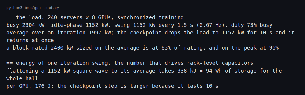
The hall swings by 1,152 kW every 1.5 s. A block rated at 2,400 kW sized on the average load of 1,997 kW looks like 83 percent loaded. On the peak of 2,304 kW it is at 96 percent. A source sized on the average would be over its rating on every compute phase.
Flattening the swing to the average takes 338 kJ of storage, which is 94 Wh for the whole hall and 176 J for each GPU. That is the energy of one iteration.
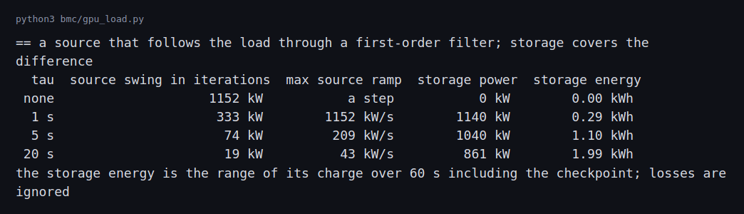
With no smoothing the source sees the whole 1,152 kW as a step in every iteration, and the checkpoint is another step. With a 1 s time constant the source still swings by 333 kW inside an iteration and ramps at up to 1,152 kW/s. With 5 s the swing is 74 kW and the fastest ramp is 209 kW/s. With 20 s it is 19 kW and 43 kW/s.
The storage pays for this. Its power is 1,140, 1,040 and 861 kW for the three settings, and its energy range over the 60 s is 0.29, 1.10 and 1.99 kWh. The iteration swing itself is only 94 Wh. Most of the energy is the checkpoint, where the load drops by 1,152 kW for 10 s and the smoothed source takes seconds to follow it.
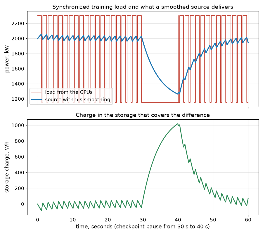
The red trace is the load, with the 0.67 Hz swing and the 10 s pause. The blue trace is the source, which barely moves during iterations and glides down and up around the checkpoint. The lower plot is the storage, which moves by tens of watt-hours each iteration and by about a kilowatt-hour over the pause.
Sizing the storage and choosing where it sits
The results above are power-bound. At the 5 s setting the storage must deliver 1,040 kW but only about 1.10 kWh of energy swing over a minute. That is a power-to-energy ratio of about 945 per hour, or a 945 C rate in battery terms. The previous post put a UPS battery behind the critical load, and a battery sized for 5 minutes of full load is a very different sizing problem. The two numbers sit in different places in a datasheet.
Cycle count decides the technology. One iteration every 1.5 s is 57,600 charge-discharge cycles a day, about 21 million a year, each only a few watt-hours deep. Typical lithium battery datasheets quote cycle life in the thousands of full-depth cycles, and typical supercapacitor datasheets quote hundreds of thousands to about a million. Those are generic ranges and the specific product’s datasheet governs. If my range is wrong for a product, the product’s rating is the one that counts. On those ranges, a lithium battery at a 2 C discharge rate would need about 520 kWh of nameplate to deliver 1,040 kW, 470 times the energy the smoothing uses, and the shallow cycling still reaches its cycle life within a year or so. A capacitor or supercapacitor bank sized at a few kWh matches the duty, which is why the production mitigations in the Differences section put capacitors in the power supplies and use batteries for the slower checkpoint part.
Split by time scale.
| Time scale | Event in this example | Where it is handled | Why |
|---|---|---|---|
| Under about 1 s | GPU step inside an iteration, 1,152 kW | Capacitors in the server power supply, GPU power-smoothing firmware | Energy is only 94 Wh for the hall, and the cycle count rules out batteries |
| 1 to 20 s | The filter’s ramp at the source, 209 kW/s at 5 s | Supercapacitors or a fast battery at the UPS DC bus or the LV bus | Power-bound, cycle-heavy duty |
| Tens of seconds | Checkpoint pause, about 1 kWh swing over 10 s | Battery energy storage or the UPS battery inverter | The energy is larger and the cycle count is a few per hour |
| Minutes and above | Generator start, peak shaving | UPS battery, site BESS | Energy-bound duty |
Where it sits on the single-line diagram.
- Inside the rack or power shelf. Fastest response and smallest bus to coordinate, but it is limited in energy and it ties the design to one vendor’s equipment.
- At the UPS DC bus. The UPS can supply a ramp-limited input while the DC link absorbs the swing. The limit is the UPS maker’s ability to hold the input ramp and its warranty terms for that duty.
- On the LV bus, behind its own breaker. Neutral to the UPS, but it adds a source to the short-circuit and arc-flash studies of the earlier posts.
- On the MV bus. Serves several blocks and also smooths for the utility, but the response seen at the rack is slower and the utility interconnection has to accept it.
What the generator and utility see. Smoothing matters at the source because a generator’s governor and voltage regulator cannot follow a 1,152 kW step every 1.5 s, and a utility may set a ramp rate or an oscillation limit. The Microsoft write-up cited below gives those limits in megawatts per second and a frequency band. Converting a requirement to my numbers is arithmetic: a limit of 100 kW/s means the 5 s setting at 209 kW/s still fails and the 20 s setting at 43 kW/s passes, with the 20 s setting needing 861 kW and 1.99 kWh of storage. The limit depends on the site, and the utility’s actual number replaces my 100 kW/s example.
Challenges
- The average load hides the peak. A UPS or generator chosen on the average load runs above its rating on every compute phase. The block rating has to cover the peak, and the redundancy post’s loading figures are peak figures for this kind of hall.
- The biggest steps are not in the iterations. The checkpoint drops the whole hall by 1,152 kW at once and brings it back at once. Job starts and stops are bigger still, and operators stagger them where they can.
- Slow meters do not see the swing. A meter that averages over a minute shows 1,997 kW and nothing else. Seeing a 0.67 Hz swing needs sampling faster than every 0.75 s, and most building meters are slower.
- The source can have limits of its own. Utilities can set limits on ramp rate, dynamic range and oscillation in a band of frequencies, and a generator has a limit on how much load it can take in one step. A hall that meets its rating can still violate these.
- Smoothing costs something. Storage has losses and a charge to manage, and smoothing in the GPUs can mean holding power up when the GPUs have nothing to do. Both use energy.
Differences with a production setup
Where a measurement, a standard, a datasheet or a vendor rating disagrees with a number in this post, the number in this post is the one that is wrong. The values most likely to differ are the square-wave profile, the 176 J per GPU and the first-order filter standing in for a real source.
- Real profiles. The load comes from measuring the actual job, its phases and the power of each GPU model. My square wave has one level for compute and one for the wait. Real jobs differ by model, parallelism scheme and hardware.
- Real requirements. Utilities and equipment makers define limits that depend on the site. Microsoft’s write-up on power stabilization for AI training datacenters lists a ramp rate in megawatts per second, a dynamic power range and limits on oscillations in a band such as 0.1 to 20 Hz, and says the limits vary with the utility and its generation equipment. My 0.67 Hz swing is inside that band.
- Mitigations in practice. The same write-up describes smoothing in the GPUs and storage outside them. NVIDIA’s blog on the GB300 NVL72 describes power supplies with 65 joules of capacitor storage per GPU and reports a 30 percent cut in peak grid demand when training a Megatron model. My 176 J per GPU is for a different profile and a different goal, so the two figures are not comparable. Neither figure is a measurement of a specific product.
- Dynamic studies. A real study models the source with its controls, the UPS with its limits and the network, in an electromagnetic transient tool such as PSCAD. A first-order filter is only a stand-in for that.
- Storage choice. Batteries, supercapacitors and capacitor banks suit different time scales, and a real design combines them. The sizing section above sizes the fast part and compares placements.
- Generator behavior. Step-load capability and the response of the governor and voltage regulator are in the maker’s data. The UPS post covers generator step-load acceptance.
FAQ
Why do all the GPUs change power at the same time?
They work on one job. Each step needs results from all the others, so they compute together and then wait together.
Why is the average load not enough for sizing?
Equipment has to carry the peak. A source sized for the average is over its rating whenever the hall is busy.
What does a longer filter time constant do?
It makes the source change more slowly, so it sees less of the swing. The storage then covers more, and it has to be bigger for slow events such as the checkpoint.
Why is the checkpoint a problem for the storage?
The load stays low for 10 s, and the smoothed source takes seconds to follow it down, so the storage absorbs the difference for that long. That makes it the largest energy in the run.
Does the UPS see these swings?
A UPS in double-conversion mode supplies the swing from its inverter, and what reaches the source depends on the input stage and the storage. UPS input-ramp limits and control response come from the maker and are an input to the transient study.
What will change the most between this model and a real GPU cluster?
The load profile. The power profile of a real training job measured on real GPUs, and the design of the storage, decide the size and timing of the swings that the model only estimates.
Repeating with real hardware
Coming soon. With a GPU server and a power meter that samples at 1 Hz or faster, I could record the real profile of a training job and run it through the same model in place of my square wave.
Next
Take the quiz to test your understanding: Electrical series quiz
The next post in this series covers on-site generation: engines, turbines and fuel cells, unit counts, availability, emissions permits and a phased build.
Comments